Monitors and Live Plotting

Keeping track of your model's performance is essential for debugging and evaluation. OpenDeep provides a flexible way to monitor variables and expressions that you may care about with three classes:

Monitor (opendeep.monitor.monitor)
MonitorsChannel (opendeep.monitor.monitor)
Plot (opendeep.monitor.plot)

In this guide, we will go over the usage of these three classes and show an example plotting train cost, classification error, and mean weights for a simple MLP.

Monitor (opendeep.monitor.monitor)

The Monitor class is the basis for indicating what variables and expressions you want to see.

It is defined by a name, expression to evaluate, and three flags (train, valid, test) to indicate which subsets of your data to use with the monitor. By default, the train flag is true while valid and test are false.

from opendeep.monitor.monitor import Monitor

your_monitor = Monitor(
  name="informative_name",
  expression=theano_expression_or_variable,
  train=True,
  valid=False,
  test=True
)

MonitorsChannel (opendeep.monitor.monitor)

The MonitorsChannel is a logical grouping of Monitor objects. It acts as an organizational helper. You can think of these channels as figures or plots, where the individual monitors in the channel are plotted in the same figure.

It is defined by a name and list of monitors, and has helper functions for accessing or modifying its monitors:

from opendeep.monitor.monitor import MonitorsChannel

# you can instantiate with a list of monitors, or add them later.
# instantiate with list:
your_channel = MonitorsChannel(
  name="your_channel_name",
  monitors=[monitor_1, monitor_2]
)

# adding monitors
your_channel.add(monitor_3)
your_channel.add([monitor_4, monitor_5])

# accessing (and removing) a monitor with a specific name from the channel:
monitor_4 = your_channel.pop("monitor_4_name")
# or just removing
your_channel.remove("monitor_3_name")

# getting the list of monitor names
monitor_names = your_channel.get_monitor_names()
# getting the list of monitor expressions
monitor_expressions = your_channel.get_monitor_expressions()

# getting the Monitor objects that should be evaluated on the train subset
train_monitors = your_channel.get_train_monitors()
# for valid subset
valid_monitors = your_channel.get_valid_monitors()
# for test
test_monitors  = your_channel.get_test_monitors()

# accessing Monitors from multiple data subsets at once (where Monitors are not duplicated)
train_and_test = your_channel.get_monitors(train=True, test=True)
valid_and_test = your_channel.get_monitors(valid=True, test=True)
# or just return them all!
all_monitors = your_channel.get_monitors()

Plot (opendeep.monitor.plot)

The Plot object interfaces with Bokeh-server. It uses a list of MonitorsChannel or Monitor objects to construct a separate figure for each channel, where the monitors within the channel get plotted on the figure. To use the plot, pass it to your Optimizer's train() function! If provided with just a Monitor, the plot treats it as a channel with the given monitor as the only object.

The Plot object will always have a train_cost figure to keep track of your training cost expression, so you never have to create a Monitor for it. The Plot is defined by:

bokeh_doc_name: name for the Bokeh document
monitor_channels: the list of MonitorsChannel or Monitor to plot
open_browser (optional): whether to open a browser to the figures immediately
start_server (optional): whether to start the bokeh server for you (not recommended, you should instead start it from the command line yourself with the command bokeh-server)
server_url (optional): the URL to use when connecting to the bokeh server
colors (optional): a list of different possible color hex codes to use for plotting (so multiple lines are legible on the same plot)

from opendeep.monitor.plot import Plot

your_plot = Plot(
  bokeh_doc_name="Your_Awesome_Plot",
  monitor_channels=[your_channel_1, your_channel_2],
  open_browser=True,
  start_server=False,
  server_url='http://localhost:5006/',
  colors=['#1f77b4', '#ff7f0e', '#2ca02c', '#d62728']
)

Example: Plotting train cost, softmax classification error, and mean weights for a simple MLP

This tutorial isn't focused on the model, so let's do something really simple. If you want an overview of the MLP, check out Classifying Handwritten MNIST Images.

from opendeep.models import Prototype, Dense, Softmax
from opendeep.optimization.loss import Neg_LL
from opendeep.optimization import AdaDelta
from opendeep.data import MNIST
from theano.tensor import matrix, lvector

# create a 1-layer MLP
mlp = Prototype()
mlp.add(Dense(inputs=((None, 28*28), matrix('xs')), outputs=512)
mlp.add(Softmax, outputs=10, out_as_probs=False)

# define our loss
loss = Neg_LL(inputs=mlp.models[-1].p_y_given_x, targets=lvector('ys'), one_hot=False)

# make our optimizer object with the mlp on the MNIST dataset
optimizer = AdaDelta(model=mlp, loss=loll, dataset=MNIST(), epochs=20)

Now our setup is out of the way, let's create some monitors and monitor channels to plot during out training!

import theano.tensor as T
from opendeep.monitor.monitor import Monitor, MonitorsChannel

# Now, let's create monitors to look at some weights statistics
W1 = mlp[0].get_params()['W']
W2 = mlp[1].get_params()['W']

mean_W1 = T.mean(W1)
mean_W2 = T.mean(W2)

mean_W1_monitor = Monitor(name="hiddens_mean", expression=mean_W1)
mean_W2_monitor = Monitor(name="out_mean", expression=mean_W2)

# create a new channel from the relevant weights monitors
weights_channel = MonitorsChannel(name="weights", monitors=[mean_W1_monitor, mean_W2_monitor])

Finally we can create a Plot object to visualize these monitors:

from opendeep.monitor.plot import Plot

# create our plot!
plot = Plot(bokeh_doc_name="Monitor_Tutorial", monitor_channels=[mlp_channel, weights_channel], open_browser=True)

# train our model and use the plot (make sure you start bokeh-server first!):
optimizer.train(plot=plot)

# that's it!

Putting it all together:

Start Bokeh server

bokeh serve

Run your python script with the model

import theano.tensor as T
from opendeep.models import Prototype, Dense, Softmax
from opendeep.optimization.loss import Neg_LL
from opendeep.optimization import AdaDelta
from opendeep.data import MNIST
from opendeep.monitor.plot import Plot
from opendeep.monitor.monitor import Monitor, MonitorsChannel

def main():
  # create a 2-layer MLP
  mlp = Prototype()
  mlp.add(Dense(inputs=((None, 28*28), T.matrix('xs')), outputs=512))
  mlp.add(Softmax, outputs=10, out_as_probs=True)

  # define our loss
  loss = Neg_LL(inputs=mlp.get_outputs(), targets=T.lvector('ys'), one_hot=False)

  # make our optimizer object with the mlp on the MNIST dataset
  optimizer = AdaDelta(model=mlp, loss=loss, dataset=MNIST(), epochs=20)

  # create the monitors and channels
  W1 = mlp[0].get_param('W')
  W2 = mlp[1].get_param('W')

  mean_W1 = T.mean(W1)
  mean_W2 = T.mean(W2)

  mean_W1_monitor = Monitor(name="hiddens_mean", expression=mean_W1)
  mean_W2_monitor = Monitor(name="out_mean", expression=mean_W2)

  weights_channel = MonitorsChannel(name="weights", monitors=[mean_W1_monitor, mean_W2_monitor])

  # create the plot
  plot = Plot(bokeh_doc_name="Monitor_Tutorial", monitor_channels=weights_channel, open_browser=True)

  # train our model!
  optimizer.train(plot=plot)


if __name__ == '__main__':
    main()

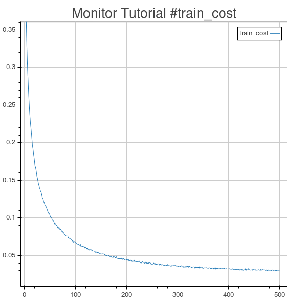
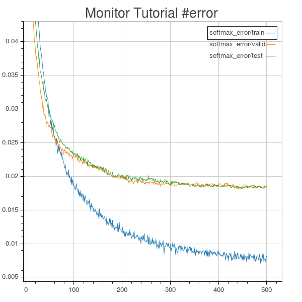
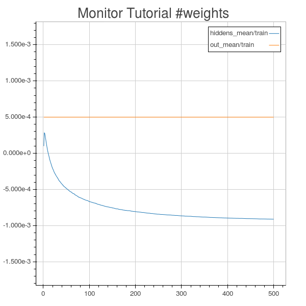
Congrats! You should get output graphs similar to the following (these were created with slightly different code):